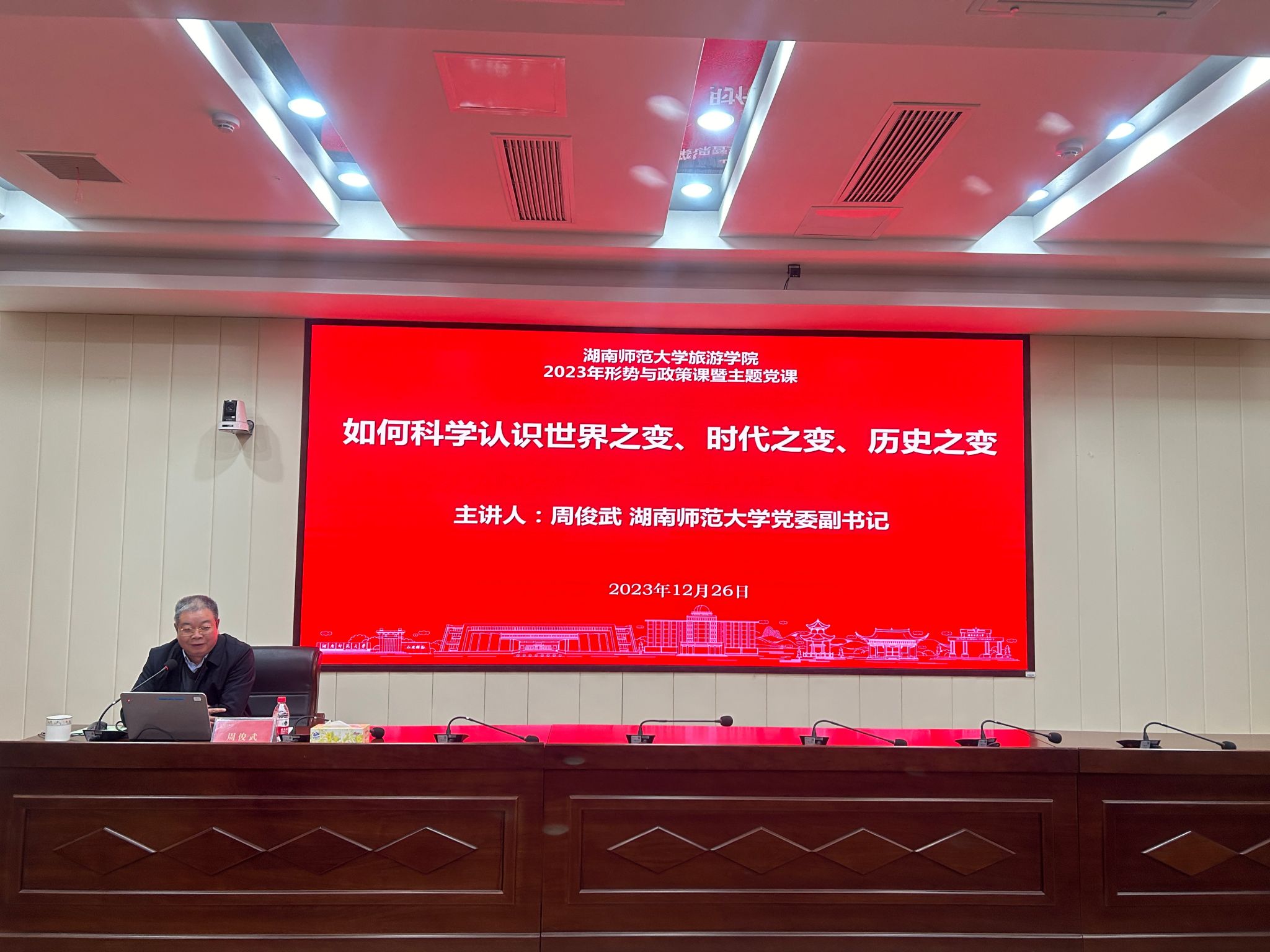
校党委副书记周俊武教授来院讲授“形势与政策”课
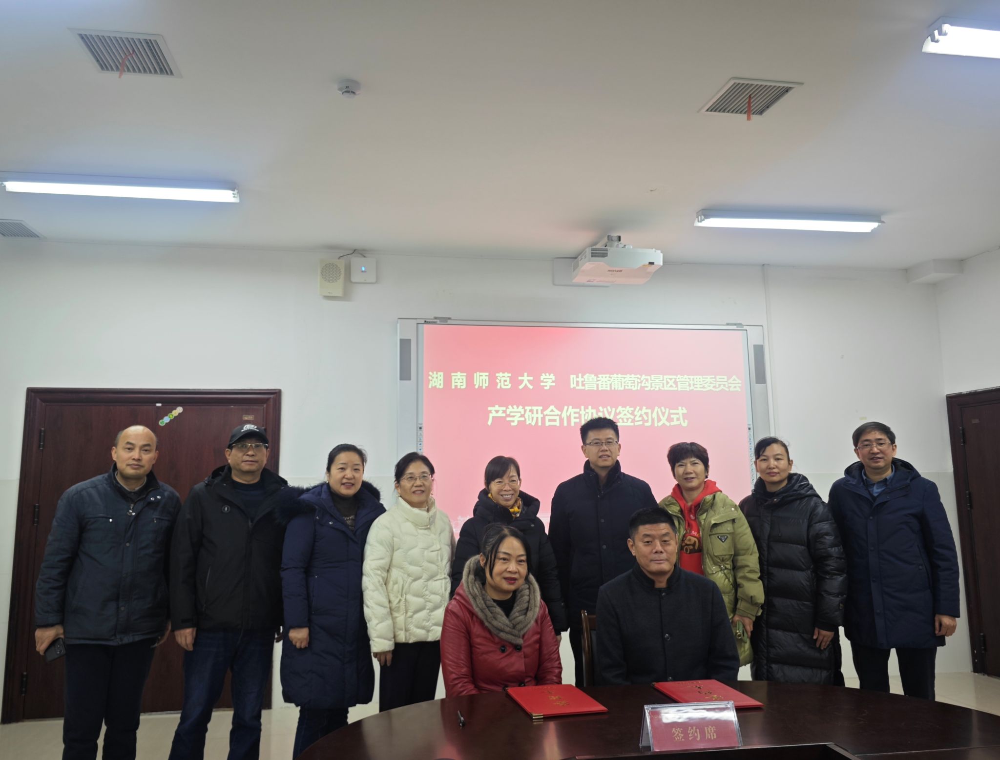
我院与吐鲁番葡萄沟景区管委会举行产学研合作签约仪式
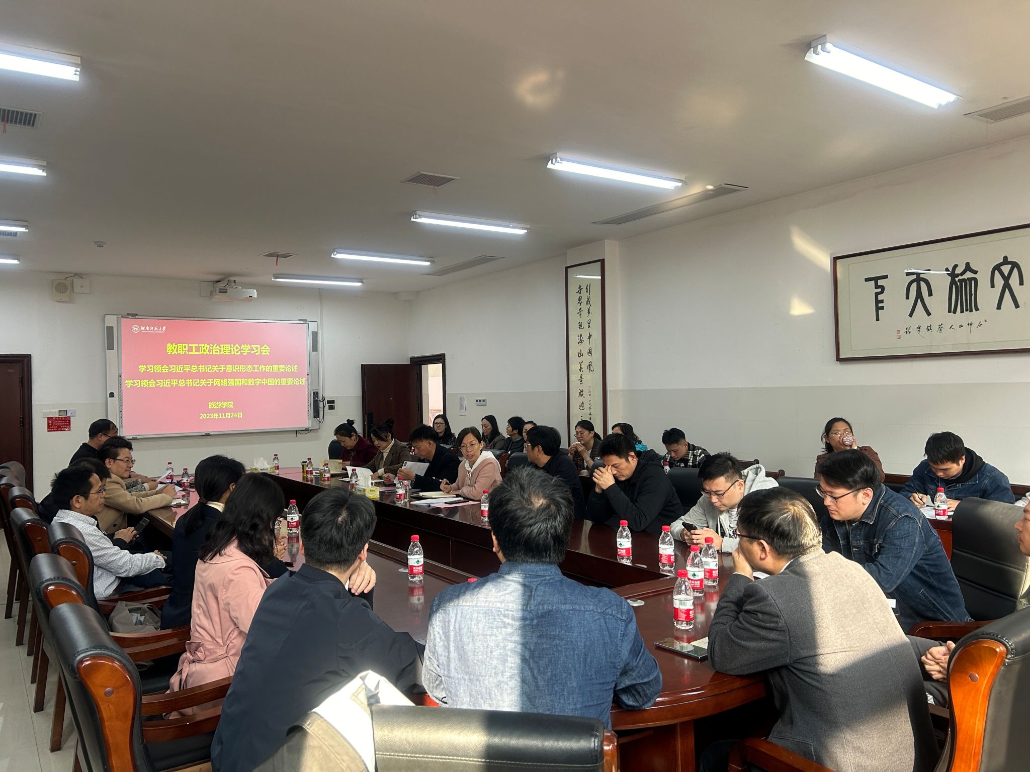
我院开展教职工政治理论学习会
我院旅游管理专业开展专业自评专家组现场考查评估
我院承办的惠州市惠阳区幼儿园骨干教师能力提升培训班顺利开班
我院承办的铜鼓县文旅人才综合能力提升培训班顺利开班
大力弘扬教育家精神——学院党委中心组专题学习习近平总书记教师节重要指示精神
伟德国际1946备用网站2023年专任教师公开招聘公告(第二批)
2023年旅游管理专业学位硕士(MTA)招生指南
2023年9月伟德国际1946备用网站伟德国际1946备用网站接受同等学力人员申请硕士学位招生简章
伟德国际1946备用网站2023年管理和教辅人员公开招聘公告
旅游管理系召开专业自评工作会议
我院应邀出席2023粤港澳暨东盟旅游研究与人才培养论坛
我院学子在第十七届全国高校商业精英挑战赛会展专业创新创业实践竞赛全国总决赛中荣获佳绩
《地理科学》高级编辑张慧敏博士为我院开展线上讲座
伟德国际1946备用网站举办《文旅新场景》公开课展示活动
上海师范大学伟德国际1946备用网站副教授张圆刚来我院讲学
海南师范大学程叶青教授为我院研究生线上讲学
我院举办“地理学论文写作规范与常见问题”学术讲座
北京第二外国语学院邹统钎教授为我院研究生线上讲学
我院青年教师在旅游学科国际顶级期刊《Tourism Management》发表文章
【红网】用创新思维助推魅力韶山红色旅游升级
【红网】用好生态资源 助力生态旅游发展
【长江日报--长江网】湖南:深入发掘长江文化的时代价值
【红网】湖南师大MTA研究生赴韶山开展研学实践活动
【新湖南】2023年“湖南旅游集团杯”全国高校商业精英挑战赛会展专业创新创业实践竞赛湖南省决赛闭幕
2023级年级大会暨考试动员会顺利召开
黄艳为我院2023级学生讲授“形势与政策”课
我院青工部开展少年儿童图书馆志愿活动
一“研”为定——我院开展2024届毕业生考研慰问活动
我院青工部开展“爱心包裹,温暖行动”志愿者活动
我院召开2024届本科毕业生就业工作动员大会
重磅官宣:伟德国际1946备用网站伟德国际1946备用网站形象片《远方》
我院举行开元森泊旅业集团2022年管培生线上招聘推介会
我院新增会展传播学交叉学科硕士点正式开始招生
我院召开2018级毕业就业家长推进会


 常用链接
常用链接


